Data Preprocessing
Before we can train any Machine Learning model, we need to deal with the messy reality of raw data. Data preprocessing is the process of transforming raw data into a clean, usable format before feeding it into a model. Think of it like washing and chopping vegetables before cooking. You can't make a good dish with dirty, uncut ingredients.
Raw data typically suffers from problems like outliers, missing values, meaningless combinations, and inconsistent scales. Preprocessing turns that chaos into something a model can actually learn from.
The 7 Steps of Data Preprocessing
Step 1 — Acquire the dataset. Gather data from various sources and combine them into a proper format. The structure of your dataset will depend on your domain (business data looks very different from medical data).
Step 2 — Import crucial libraries. In Python, three libraries form the backbone of preprocessing: NumPy (scientific computing), Pandas (data manipulation and analysis), and Matplotlib (2D plotting and visualization).
Step 3 — Import the dataset. Load your data into your working environment. Make sure your working directory is set correctly so your code can find the files.
Step 4 — Handle missing values. This is critical. If you ignore missing data, your model will draw faulty conclusions. Common strategies include filling missing values with the column mean/median, or dropping incomplete rows entirely.
What's imputation (filling in) and dropping (removing row)?
Imagine a spreadsheet of patient records where some rows have no entry for "blood pressure." If you feed that gap straight into a model, it either crashes or silently learns something wrong. You have two main options: imputation (filling in a reasonable substitute) or deletion (removing the incomplete row).
For imputation, the most common approach is replacing the blank with the column's mean or median. Mean works well for normally distributed data, while median is safer when you have outliers — for instance, if most blood pressures are around 120 but one reading is 300, the mean gets pulled up, while the median stays stable. Deletion is simpler but risky: if 30% of your rows are missing that field, you're throwing away a lot of data.
Step 5 — Encode categorical data. ML models run on math — they need numbers, not labels like "Red" or "Male." Encoding methods include dummy variables, label encoding (assigning integers to categories), and one-hot encoding (creating binary columns for each category).
Label encoding vs one-hot encoding
Models do math, so a column like "Color" with values Red, Blue, Green is meaningless to them as text. Label encoding assigns each category an integer (Red=0, Blue=1, Green=2), which is quick but introduces a problem: the model may interpret Blue as "between" Red and Green, or assume Green > Red, when there's no such ordering.
One-hot encoding avoids this by creating a separate binary column for each category, so you'd get three columns (is_Red, is_Blue, is_Green), each containing 0 or 1. The trade-off is that one-hot encoding adds more columns, which can be expensive with high-cardinality features (imagine a "City" column with 500 unique values).
Step 6 — Feature scaling. When your features have wildly different ranges (e.g., age 0–100 vs. salary 0–1,000,000), some algorithms get confused. Feature scaling standardizes variables to a common range. Two popular methods are Min-Max scaling and Standardisation (z-score).
Feature scaling
Say you have two features: age (ranging 18–65) and income (ranging 20,000–200,000). A distance-based algorithm like k-nearest neighbours calculates how "close" two data points are. Without scaling, income dominates that distance calculation simply because its numbers are bigger — age differences become basically invisible. Scaling fixes this by putting both features on a comparable range.
Min-Max scaling squeezes everything into 0–1 using the formula
Not all algorithms need feature scaling. Tree-based models (like decision trees and random forests) split on thresholds and don't care about magnitude, so scaling doesn't affect them. It matters most for distance-based and gradient-based algorithms.
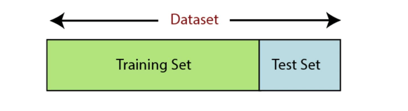
Step 7 — Split the dataset. Divide your data into a training set (for learning) and a test set (for validation). Common splits follow the Pareto principle: 80/20, 70/30, or 60/40.
Other Preprocessing Techniques
Beyond the core 7 steps, you may also encounter:
- Data Integration — combining data from multiple source systems into a unified set.
- Data Transformation — converting data from one format to another (e.g., source system format → destination format).
- Data Discretization — turning continuous values into discrete intervals (e.g., converting exact ages into age groups like "18–25", "26–35").
Regression Analysis
Now that our data is clean, let's learn how to make predictions. We'll start with a classic example.
The Housing Price Problem
Imagine we have a dataset of 47 houses in SS17, Petaling Jaya, with their living areas (in square feet) and prices (in RM thousands). The question is simple: given the size of a house, can we predict its price?
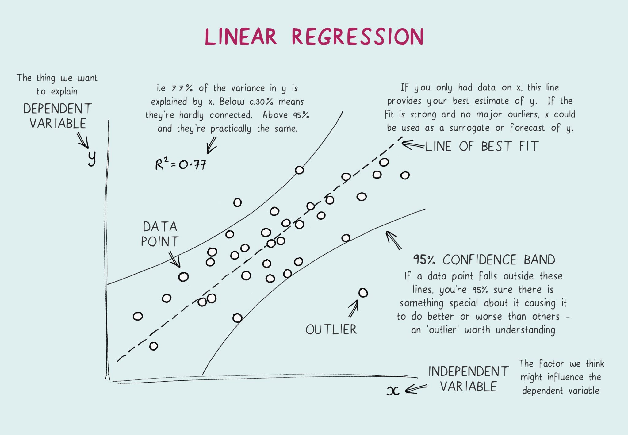
This is a supervised learning problem. We have input-output pairs and want to learn a mapping between them. Since the output (price) is a continuous value, this is specifically called a regression problem.
Regression is a method for finding the relationship between variables so you can predict a continuous outcome from one or more inputs.
Notation
Before diving in, let's set up our notation:
= input features (e.g., living area of the i-th house) = output/target variable (e.g., price of the i-th house) = a single training example = total number of training examples = our hypothesis function — the predictor we want to learn
The goal: learn a function h such that
Linear Regression
The simplest hypothesis is a linear function. If we have two features — living area (
The
The Cost Function
We define a least-squares cost function that measures how far off our predictions are from the actual values:
The smaller
Recap Cost Function
You can learn more about cost function here. The core idea remains pretty much the same, only difference is that this formula writes the cost as the sum of all errors, which corresponds to batch gradient descent where you accumulate the total error across every example before making one update. Batch is more stable per step, but each step is expensive because you have to loop through the entire dataset.
Gradient Descent — Finding the Best Parameters
Gradient descent is an iterative optimization algorithm. Here's the intuition:
- Start with a random guess for
. - Compute the cost
. - Adjust
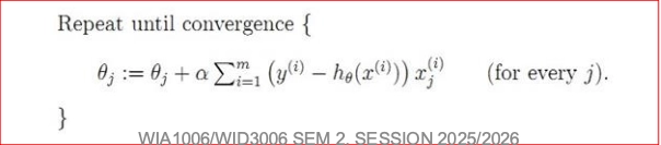
in the direction that reduces the most (the direction of steepest descent). - Repeat until convergence. The update rule is:
Understanding the formula
This is gradient descent in its simplest form, adjust the weight by stepping in the opposite direction of the slope, using a small learning rate so we don't overshoot. If you want to learn more, check out this post, but just note that it's the same update rule, just applied in a deeper context. Linear regression uses the simplest form of this update, back-propagation extends it to networks with multiple layers.
Here,
Working out the partial derivative, the update becomes:
This is called the LMS (Least Mean Squares) update rule, also known as the Widrow-Hoff learning rule. Notice something elegant: the size of the update is proportional to the error. When the prediction is close to the actual value, the adjustment is tiny. When the error is large, the adjustment is large.
Deriving the equation
The goal is to find the partial derivative for our update rule:
We start with our Least Squares Cost Function (summing over all
And our linear hypothesis:
Set up the Explicit Chain Rule
Instead of differentiating everything at once, we split the derivative into two clear parts using Leibniz notation:
We put the derivatives inside the sum because the total gradient is just the sum of the gradients of each individual training example.
Calculate the Two Parts
Part 1: How does the cost change with respect to the prediction?
Let
Part 2: How does the prediction change with respect to the weight
Combine the Chain Rule
Now, we multiply Part 1 and Part 2 together and place them back inside our summation:
The Final Update Rules
Substitute the combined derivative back into the original gradient descent update rule:
To get the most elegant form, distribute the negative sign to flip the inner terms
For Batch Gradient Descent (All Samples):
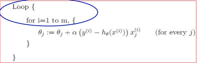
For Stochastic Gradient Descent (1 Sample at a time): We simply drop the summation, giving us the exact LMS update rule:
Batch vs. Stochastic Gradient Descent
Batch Gradient Descent sums the gradients over all training examples before making a single update. It's precise but can be slow for large datasets.
Stochastic (Incremental) Gradient Descent updates
Underfitting vs. Overfitting
This is one of the most important concepts in ML. Consider fitting different models to our housing data:
- A straight line (linear fit) may be too simple — it doesn't capture the curve in the data. This is underfitting.
- A quadratic (adding
) fits better, capturing more structure. - A 5th-order polynomial passes through every data point perfectly, but it would make terrible predictions on new data. This is overfitting.
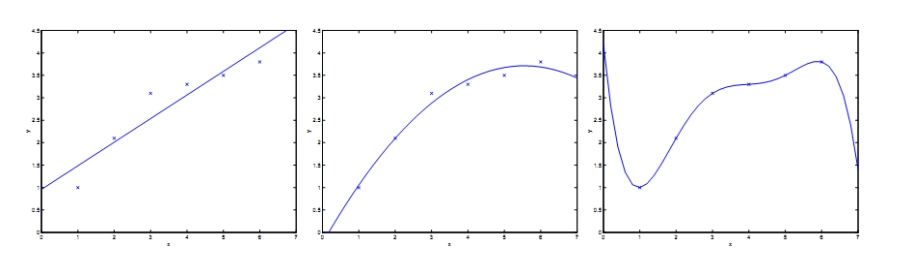
The key insight: a model that memorizes training data is not necessarily a good model. We want one that generalizes to unseen data.
Locally Weighted Linear Regression
Standard linear regression fits one global line to all data. Locally Weighted Linear Regression (LWLR) takes a different approach: for each prediction, it gives more importance to nearby training points and less to distant ones.
The weight for each training example is typically a Gaussian function:
The parameter
The Intuition behind Locally Weighted Linear Regression (LWLR)
In standard linear regression, when you fit a line, every single training example has an equal vote. A house that is 5,000 sq ft has the exact same influence on the line as a house that is 1,000 sq ft.
LWLR changes this. If you want to predict the price of a house that is 1,500 sq ft (your query point,
To do this, we multiply the error of each training example by a weight,
Deconstructing the Equation
The weight formula is a Gaussian (bell-shaped) curve:
Here is what each piece is doing:
- The Distance:
This is the squared distance between a training exampleand the specific point you are trying to predict . - If the training point is very close to your query point, this value is almost 0.
- If the training point is very far away, this value is large.
- The Exponential & Negative Sign:
Because of the negative sign, we are doingto the power of a negative number. - If the distance is roughly
(the points are close), we get . The weight is . The model gives this point maximum importance. - If the distance is large (the points are far), we get
, which approaches 0. The weight becomes . The model completely ignores this point.
- If the distance is roughly
- The Bandwidth Parameter:
(Tau) dictates how "fat" or "thin" our bell curve is. It controls how quickly the weights fall off to zero as you move away from the query point . - Large
: The weights fall off very slowly. The model looks at a very wide "neighborhood" of points. If is infinitely large, LWLR just becomes standard linear regression. - Small
: The weights fall off rapidly. The model only looks at a very tiny, strict neighborhood of points immediately next to .
- Large
Why is it called "Non-parametric"?
Standard linear regression is parametric. You look at the data once, calculate your
LWLR is non-parametric. Because the weights
Logistic Regression
Everything above assumes y is continuous. But what if y can only be 0 or 1 (e.g., spam vs. not spam, tumor is malignant vs. benign)?
We can't use a plain linear function because it can output values outside 0, 1. Instead, we wrap it in the sigmoid (logistic) function:
The sigmoid squashes any real number into the range (0, 1), which we interpret as a probability. If
The Problem with Linear Regression for Classification
Imagine you are a doctor trying to predict if a tumor is Malignant (
If you use standard Linear Regression, you fit a straight line through the data. You might say: "If the line outputs a value greater than 0.5, I will predict 1 (Malignant). If it's less than 0.5, I predict 0 (Benign)."
This works okay until a patient comes in with a massive tumor.
Because linear regression is a straight line, it will try to accommodate this massive outlier. The line will tilt upwards heavily. Suddenly, your
Even worse, the straight line might output a value like
The Solution: The Sigmoid Function
Instead of a straight line, we want a curve that flatlines at
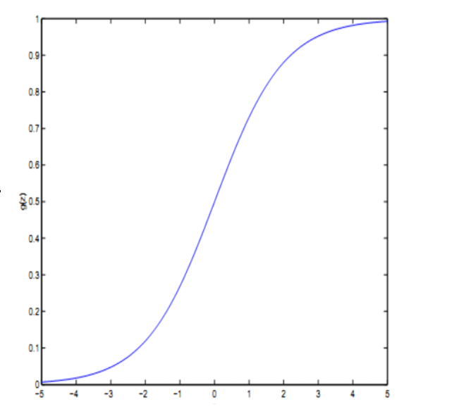
This is what the Sigmoid function does:
Think of
- If the raw score is
, the sigmoid turns it into exactly (50% probability). - If the raw score is a huge positive number (like
), the sigmoid squashes it to (99.99% probability it is Malignant). - If the raw score is a huge negative number (like
), the sigmoid squashes it to (0.01% probability it is Malignant).
Logistic Regression is just Linear Regression wrapped in a translator that turns "raw scores" into "probabilities."
Fitting Logistic Regression
Instead of minimizing squared error, we use maximum likelihood estimation. We assume:
The log-likelihood is:
We maximize this using — you guessed it — gradient descent. The resulting update rule looks remarkably similar to the linear regression one:
The form is identical, but remember that h(x) is now the sigmoid function, not a linear function. This elegant symmetry is one of the beautiful things about these algorithms.
The Log-Likelihood Cost Function
In Linear Regression, we used the Least-Squares cost function (minimising the squared error). Because the prediction is just a straight line, Least-Squares naturally creates a perfect "U-shaped" error graph (a parabola)
But if we try to use Least-Squares for Logistic Regression, we have to shove the complicated Sigmoid fraction
The math breaks. The
Maximum Likelihood Estimation
Because we are dealing with 0s and 1s, statisticians stopped measuring "distance" (Least Squares) and started measuring "probability".
If you want to know the total chance that your model predicted Patient 1 correctly (90% sure) AND Patient 2 correctly (80% sure), you multiply the probabilities together:
This is called Maximum Likelihood. We want the model to adjust its weights to make the final multiplied success rate as high as absolutely possible.
Summoning the Logarithm
There is one problem: if you multiply 10,000 probabilities together (
To stop the computer from crashing, we wrap the whole thing in a logarithm. A magical rule of math is that
The Log-Likelihood Cost Function
This brings us to the actual cost function:
This terrifying equation is actually just an elegant logical "IF" statement:
- If the actual answer is
: The second half of the equation becomes and disappears. We are just left with . We want our prediction to be as close to as possible. - If the actual answer is
: The first half of the equation becomes and disappears. We are left with . We want our prediction to be as close to as possible.
Because of the logarithm, the model is heavily punished if it is confidently wrong. (e.g., If it predicts a 99% probability of a tumor being Malignant, but it's actually Benign, the error slope becomes a massive cliff, screaming at the model to turn around).
Statisticians didn't add the log to fix the bumpy error graph, they added it so computers wouldn't crash.
However, because the Sigmoid formula relies on an exponential (
It magically ironed out the flat spots and local minima, turning the error graph back into a perfect, smooth U-shape bowl.
Summary
| Topic | Key Idea |
|---|---|
| Data Preprocessing | Clean and transform raw data before training |
| Linear Regression | Predict continuous values with a linear model |
| Cost Function (J) | Measures how wrong our predictions are |
| Gradient Descent | Iteratively adjust parameters to minimize cost |
| Batch vs. Stochastic GD | Update after all examples vs. after each example |
| Underfitting / Overfitting | Too simple vs. too complex models |
| Locally Weighted LR | Give nearby points more influence |
| Logistic Regression | Classify discrete outcomes using the sigmoid function |