1. The Paradigm Shift: Why Artificial Neural Networks?
For decades, computing has been dominated by the Von Neumann architecture, a design predicated on sequential processing, explicit memory addressing, and rigid algorithmic logic. While highly effective for arithmetic calculations and strictly defined logical operations, the Von Neumann model struggles profoundly with tasks that humans find trivial, such as:
- Pattern Recognition: Identifying faces, deciphering handwritten characters, or processing natural speech.
- Content-Addressable Recall: Retrieving complex memories based on partial cues rather than explicit memory addresses.
- Approximate Reasoning: Making common-sense decisions in ambiguous, ill-defined environments (e.g., driving a car, playing a sport).
These tasks are difficult to program algorithmically because they rely on experience, adaptation, and the ability to tolerate noise, rather than rigid mathematical logic. To solve these problems, computer science draws inspiration from the human brain, leading to the development of Artificial Neural Networks (ANNs).
Biological Neural Networks (BNN) vs. Von Neumann Machines
The fundamental difference between biological brains and traditional computers lies in their architecture and processing methods.
| Feature | Von Neumann Machine | Human Brain (Biological Neural Network) |
|---|---|---|
| Processors | One or a few high-speed processors (nanosecond operations). | Billions ( |
| Computing Power | Massive power concentrated in localized CPU units. | Limited individual power, relying on massive collective parallelization. |
| Connectivity | Shared, high-speed buses routing data sequentially. | Massive interconnections ( |
| Memory Access | Sequential access via explicit physical addresses. | Content-addressable recall (retrieval by association). |
| Knowledge Storage | Knowledge and problem-solving logic are explicitly separated from the computing hardware. | Knowledge is distributed and physically resides in the synaptic connectivity between neurons. |
| Adaptability | Hard-coded and rigid; highly susceptible to catastrophic failure if hardware is damaged. | Highly adaptive; learns by altering network connectivity. Exhibits graceful degradation if partially damaged. |
BNN vs. ANN
While ANNs are inspired by biological brains, the practical engineered version is a tiny, brittle imitation of the real thing. The slides include this distinct comparison:
| Feature | Biological Neural Network (BNN) | Artificial Neural Network (ANN) |
|---|---|---|
| Parallelism | Massively parallel, slow per neuron, but superior overall | Massively parallel, fast per node, but inferior overall |
| Scale | ~ | Typically |
| Ambiguity | Tolerates ambiguity natively | Requires precise, structured, formatted data to handle ambiguity |
| Fault tolerance | Performance degrades gracefully under partial damage | Robust performance is possible but not automatic |
| Information storage | Stored in the synapses (the connections themselves) | Stored in continuous memory locations |
The takeaway: ANNs borrow the idea of distributed parallel computation, but they're orders of magnitude smaller and far less robust than the biological systems that inspired them.
2. From Biological to Artificial Neurons
To engineer an ANN, we must abstract the biological mechanisms of the brain into mathematical models.
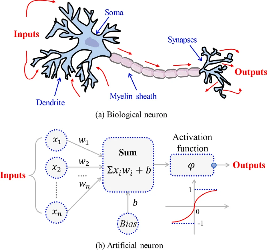
The Biological Neuron
A biological neuron consists of four primary components:
- Dendrites: Branching structures that receive incoming signals from other neurons.
- Soma (Cell Body): Accumulates the incoming signals.
- Axon: A long fiber that transmits the signal outward if the accumulated stimulus exceeds a certain threshold (action potential).
- Synapse: The microscopic gap between the axon of one neuron and the dendrite of another. The efficiency (strength) of the signal exchange across this gap determines how strongly one neuron influences another.
The Artificial Neuron
The artificial neuron (often called a node, unit, or perceptron) mirrors this biological structure mathematically:
- Inputs (
): Represent the incoming signals (dendrites). - Weights (
): Represent the synaptic strength. A high weight amplifies an input; a low weight diminishes it. - Summation Function (
): Acts as the soma, computing the weighted sum of all incoming signals. - Activation Function (
): Acts as the axon, determining the final output ( ) based on the aggregated signal. It evaluates whether the "neuron" should fire.
3. Neural Network Architecture and Topology
An Artificial Neural Network is essentially a collection of these artificial neurons connected by weighted links. What a network can compute is primarily determined by its architecture and the values of its weights.
Networks are classified by several attributes:
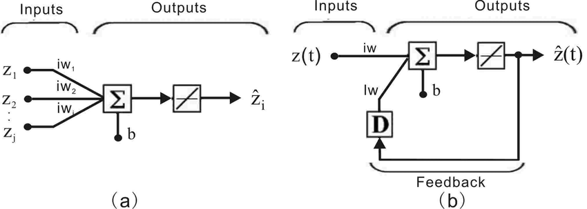
1. Connection Type
- Static (Feedforward): Signals travel in strictly one direction, from input to output. There are no loops.
- Dynamic (Recurrent/Feedback): Network connections form directed cycles. Outputs of nodes are fed back as inputs to themselves or previous layers, allowing the network to maintain an internal state or "memory" of past inputs.
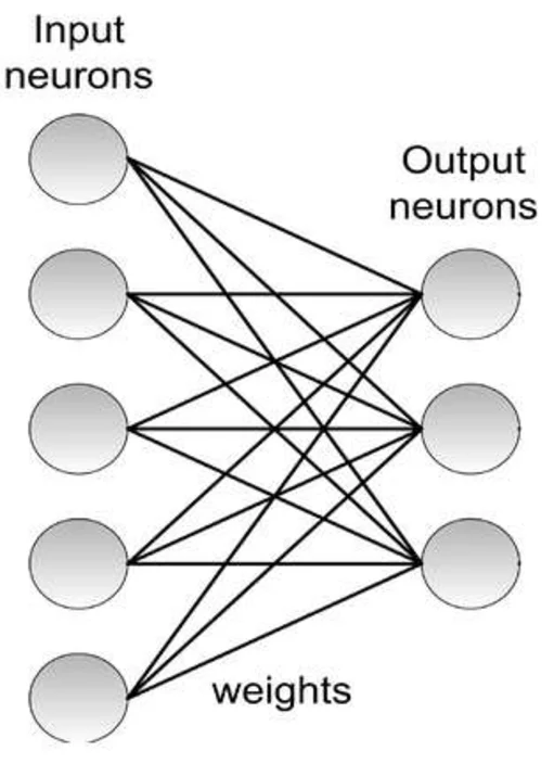
2. Topology
- Single-layer: Inputs map directly to a single layer of output nodes.
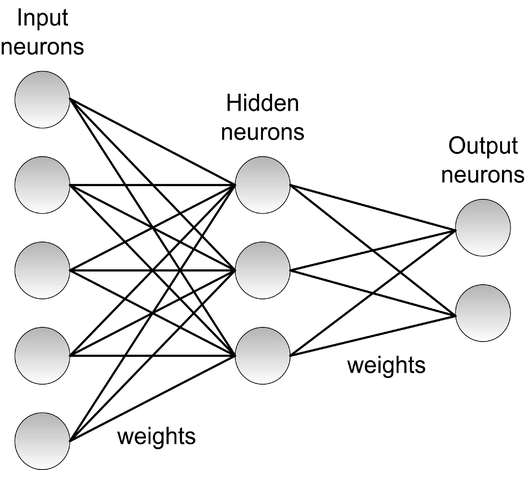
- Multi-layer: Contains one or more hidden layers between the input and output layers. This dramatically increases the representational power of the network, allowing it to learn non-linear decision boundaries.
- Self-organized: Networks that autonomously organize their topology based on data patterns (often used in unsupervised learning).
4. Learning Paradigms
For a neural network to be useful, it must "learn." Learning is the process of adjusting the synaptic weights to minimize the difference between the network's current output and the desired outcome.
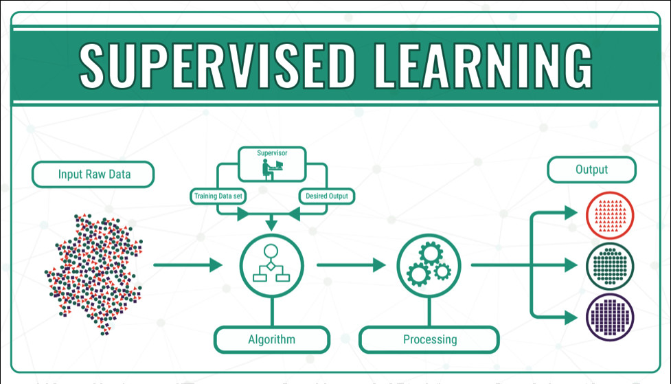
Supervised Learning: The network is provided with a training dataset consisting of paired inputs and explicit desired outputs (labels). An algorithm calculates the error between the network's prediction and the true label, adjusting the weights to correct the error.
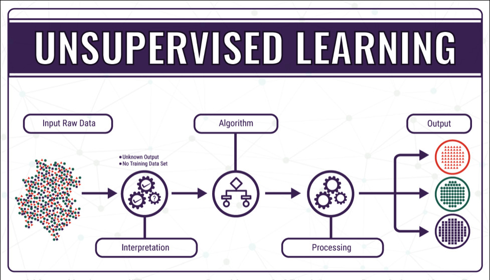
Unsupervised Learning: The network receives input data without any explicit labels. The algorithm's goal is to discover hidden structures, correlations, or natural clusters within the raw data.
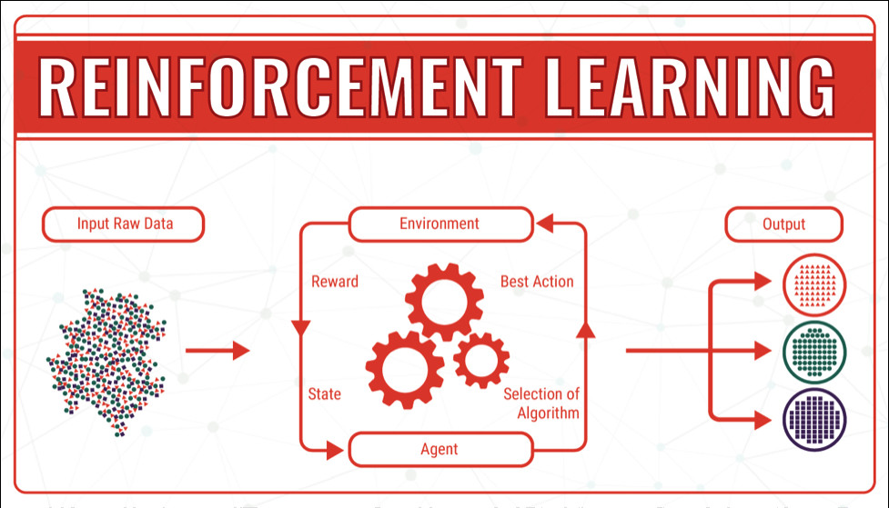
Reinforcement Learning: The network (acting as an agent) interacts with an environment. It receives positive rewards for correct actions and negative rewards for incorrect ones, adjusting its weights to maximize total cumulative reward over time.
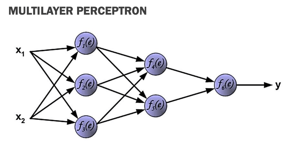
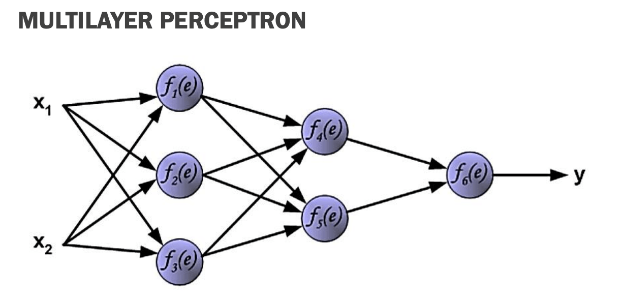
5. The Multilayer Perceptron (MLP) and Backpropagation
The most fundamental architecture for supervised learning is the Multilayer Perceptron (MLP). An MLP consists of an input layer, at least one hidden layer, and an output layer.
To train an MLP, we use the Backpropagation (BP) algorithm. Backpropagation is a gradient descent optimization technique that propagates the output error backward through the network to update the weights of the hidden layers.
The Challenge of Hidden Layers
In a single-layer network, updating weights is straightforward (using the Delta Rule) because we know the explicit target value for the output node. However, in a multi-layer network, we do not know the target output for the nodes in the hidden layers. Backpropagation solves this by calculating how much each hidden node contributed to the final output error, assigning "blame" proportionately using the chain rule of calculus.
Mathematical Notation for Backpropagation
Let us define the parameters for a network with an input layer (Layer 0), a hidden layer (Layer 1), and an output layer (Layer 2):
- Weights:
: Weight matrix from the input layer to the hidden layer. Specifically, is the weight connecting input node to hidden node . : Weight matrix from the hidden layer to the output layer.
- Training Samples: A set of
samples, denoted as . - Input Pattern (
): A vector of inputs for a given sample. - Desired Output (
): The ground truth target vector. - Actual Output (
or ): The network's calculated output vector. - Error (
): The difference between the desired and actual output for node given sample . .
The overall Objective Function is to minimize the Sum Squared Error (E) across all
Making sense of the formulas
A vector is simply a list or array of numbers arranged in a specific order.
When we train a neural network, we feed it data (inputs) and tell it what the correct answer should be (targets).
The input here is the list of features you are feeding into the network for one specific example (sample
Let's say you are training an AI to predict a house's price. Your input vector for one specific house might be: [3, 2000, 15]. This vector represents 3 bedrooms, 2000 square feet, and 15 years old. The network receives these three numbers at its input layer.
The output is a vector because the output might be more than one number. For example, an AI that's trained to classify animals as Dog, Cat, or Bird, the output layer will contain 3 nodes, [0, 1, 0] (0% Dog, 100% Cat, 0% Bird).
The Simple Error for One Node
This formula just says: Error = (What we wanted) - (What the network actually guessed). If the target was
The Big Objective Function (Sum Squared Error):
: First, calculate the error (Desired minus Output) for a specific output node. Then, square it. - Why square it? Two reasons: First, it turns negative errors into positive numbers, so a
error and a error don't accidentally cancel each other out to zero. Second, it heavily penalizes large errors (an error of 4 becomes 16, screaming at the network "FIX THIS!").
- Why square it? Two reasons: First, it turns negative errors into positive numbers, so a
: Add up those squared errors for all the output nodes ( ) in the network for that one specific sample. : Do that for every single training sample ( ) in your entire dataset, and add them all together into one giant number.
In plain English: The Objective Function (
Step 1: Forward Computing (The Forward Pass)
Data propagates forward from inputs to outputs.
Hidden Layer Calculation: The input vector
Formula explanation
The Inputs (
The Weights (
The Multiply and Add (
The Activation Function (
Output Layer Calculation: The hidden layer's output becomes the input for the output layer.
Formula explanation
This is the exact same formula as the first one. The only thing that has changed is where the data is coming from: Instead of using the raw data (
Step 2: The Activation Function (Sigmoid)
For backpropagation to work, the activation function must be non-linear and differentiable. The most common classical choice is the Logistic Sigmoid Function:
The sigmoid function maps any real-valued number into a smooth range between 0 and 1. Its most crucial mathematical property is its easily computable derivative, which is vital for the chain rule:
Deriving S'(x) step by step
We treat
The derivative of
Now split the fraction into a product:
The first factor is just
Therefore:
This is the magic property that makes sigmoid so practical: once you've computed
Note on Saturation
If the net input
Step 3: Backpropagating the Error (The Backward Pass)
We must update the weights to minimize the error
Before diving into the neural network math, let's do a quick recap on the calculus tools we need: Partial Derivatives and the Chain Rule. You can freely jump to the next section if you are already familiar with them.
Prerequisite: Partial Derivatives & The Chain Rule
Partial Derivative (
Before anything else, I think it is worth understanding how partial derivative works. We will skip the boring analogy and jump right into the math.
Let's first look at a standard derivative (
A standard derivative tells you the slope of a given equation. Take
But what if you have more than 1 variable? Take this example:
Its graph will look something like this.
It's hard to find the slope at a given point, as the you can have the slope face any direction. So we can use partial derivative here. We pretend that one of the variable is a boring, normal number (like 10).
Find the partial derivative with respect to
We pretend
If
What is the standard derivative of a plain number like
So, the derivative of
Answer:
Find the partial derivative with respect to
Now pretend
The derivative of
Answer:
In neural networks, variables are usually multiplied together (like a Weight multiplied by an Input). Let's look at a function where they are attached:
Find the partial derivative with respect to
Pretend
If
The derivative of
Now, let's swap the
Answer:
Find the partial derivative with respect to
Pretend
This means that entire chunk of
Your equation would look like this:
What is the derivative of
So, if the derivative of
Answer:
So the partial derivative essentially allows you to "lock" one of the axis by freezing all other variables. We can take a complex 3D graph, slice it into 2D cross-section, and do regular, easy standard derivative on that slice. A neural network can consists of billions of variables. Trying to comprehend a mathematical shape with a billion dimensions is literally impossible for a human brain.
Just as an example, in a network,
Then the network calculates
It does this for every single weight. Once it knows the "partial" blame for every individual weight, it adjusts them all at once, and the network learns!
The Chain rule
In calculus, the Chain Rule is a formula used to find the derivative of nested functions, meaning a function that is sitting inside another function.
A nested function looks like this:
changes changes changes
If you want to know "How much does
Updating Output Layer Weights (
To update a specific weight, we use this formula:
The Learning Rate η
The proportionality
- Too small → learning crawls; the network needs millions of epochs to converge.
- Too large → the optimizer overshoots minima, oscillates, or diverges entirely.
In code, every backprop weight update has this form:
where
Breaking down the Update Rule
Since I'm having trouble understanding the formula, so here's a very very detailed explanation:
The Left Side:
- The Triangle (
): This is the Greek letter Delta, and in math, it simply means "Change". - The Weight (
): This is the specific weight (connection) between a hidden node ( ) and an output node ( ). - Put it together: The entire left side just means: "The exact amount we need to adjust this specific weight."
The Middle:
- This symbol means "is proportional to."
- It basically means the left side scales with the right side (we can replace this symbol with an equals sign
by multiplying the right side by a small number called a "learning rate")
The Right Side:
This is the most important part, and it has two pieces: the fraction and the negative sign.
- The Fraction (
): This is the "blame." It answers the question: "If I turn this weight UP, what happens to the total Error?" - If the answer is positive (e.g.,
), it means turning the weight up makes the error worse. - If the answer is negative (e.g.,
), it means turning the weight up makes the error better.
- If the answer is positive (e.g.,
- The Negative Sign (
) [CRUCIAL!]: This is the magic of Gradient Descent. The negative sign tells the network to do the exact opposite of whatever causes more error. - If turning the weight up makes the error worse (
), the negative sign flips it to . The network says, "Okay, I will turn the weight DOWN." - If turning the weight up makes the error go down (
), the negative sign flips it to . The network says, "Great! I will turn the weight UP even more."
- If turning the weight up makes the error worse (
However, we cannot directly calculate
To bridge this gap, we use the Chain Rule. We map out the exact sequence of events that happen when a weight is tweaked: a change in the weight alters the Net Input, which alters the Output, which alters the Error.
Mathematically, we chain these three partial derivatives together:
Concept: Mapping out the Chain Rule
Let's imagine we are mathematicians trying to figure out this equation ourselves.
We have a neural network with a huge Error (
However, we can't directly calculate this because the Error formula
To connect
- Domino 1: The Weight changes the Net Input.
The weight (
) is multiplied by the incoming signal to create the net input ( ). Thus, a change in causes a direct change in . This gives us our first piece: - Domino 2: The Net Input changes the Output.
Does the
directly change the Error? No. First, it has to pass through the activation function ( ) to become the final output ( ). A change in causes a direct change in . This gives us our second piece: - Domino 3: The Output changes the Error.
Finally, the output (
) is compared to our dataset target ( ) to calculate the final Error. A change in causes a direct change in . This gives us our final piece:
We've just mapped out a composite function:
Decoding the Labels
The numbers and letters are just coordinate labels to tell you exactly where you are in the network.
- The Superscript
: This tells you which layers the weight is bridging. It means this weight connects Layer 1 (hidden) to Layer 2 (output). (Note: It is conventionally written backward as Target, Source). - The Subscript
: This tells you the specific nodes. It connects node (in the hidden layer) to node (in the output layer).
So,
Math: Solving the 3 parts of the Chain Rule
Remember that we have the blueprint equation above? Partial derivatives doesn't work well against computers, so we need to further derive the equation. So, from the steps above, we already knows these 3 formulas:
- The Error Formula:
- The Output Formula:
- The Net Input Formula:
Step 1: Solve
We want to find the derivative of the Error with respect to a specific output node
The formula:
- Freeze the other nodes: The original Error equation depends on ALL changing outputs. If your network has 3 output nodes, the formula looks like this:
We only want the partial derivative for the first node ( ). So, we lock and into place, treating them as constants. This changes the function to . - Because the derivatives of those frozen constants become
, we are left looking only at: - Apply the Power Rule: To take the derivative of something squared, we bring the
down to the front: - The Inner Chain Rule: In calculus, if you take the derivative of the outside (the square), you must multiply it by the derivative of the inside. The derivative of
(a frozen target number) is . The derivative of is . - Multiply the result by
:
Answer 1:
Some textbooks will drop the 2 in front, as it won't affect the final target (we still want error to be 0), and the 2 is absorbed into the learning rate anyways, which we will talk about later.
Why is
frozen? Remember what
actually is in the real world: it is your Desired target. It is the "ground truth" label from your dataset. If you feed the network a picture of a dog, and the label for dog is
1, then. The output (
) is going to change constantly as the network learns and tweaks its weights. But the picture is always going to be a dog. The target never changes; it is a permanent, hardcoded number for that specific training sample. Because
is just a plain, unchanging number, the rules of calculus say that its derivative is exactly .
Step 2: Solve
We want to find the derivative of the Output with respect to the Net Input.
The formula:
- This one requires almost no math!
just represents the activation function. - In calculus, the universal shorthand for "the derivative of function
" is simply writing it with a prime symbol: . - Answer 2:
Step 3: Solve
We want to find the derivative of the Net Input with respect to one specific weight.
The formula:
- Freeze the other connections: The Net Input is calculated by adding up all the incoming signals:
- Because we are taking a partial derivative for one specific weight (
), we freeze all the other weights. They turn into normal numbers without slopes, so their derivatives become . - We are left looking only at the specific piece of the formula connected to our weight:
- The Sticky Constant: Remember the rule for multiplying variables! We pretend the input (
) is a boring, frozen number like . - The derivative of
is just . Therefore, the derivative of is just .
Answer 3:
Updating Hidden Layer Weights (
This is the core of backpropagation. A hidden node
The Hidden Layer
The blueprint equation we just built above is only the simplest case. It only calculates the blame for the very last set of weights in the network (the ones touching the final Output). What if we want to calculate the blame for a weight deeper inside the network? Say, between the input layer and a hidden layer. We can apply the same logic, but we will run into two new challanges, longer chains and fork roads.
1. Longer Chains
If you are tweaking a weight deeper in the network (
Instead of a 3-step chain, you now have a 5-step chain. If you tweak a deep weight, the ripple effect looks like this:
- The Deep Weight changes the Deep Net Input.
- The Deep Net Input changes the Deep Output (the Hidden Node's signal).
- The Hidden Node's signal travels forward and changes the Final Net Input.
- The Final Net Input changes the Final Output.
- The Final Output changes the Error.
If it was just a straight line, your blueprint would just be those 5 derivatives multiplied together:
2. The Fork in the Road (Why we need the
But in neural network's context, the chain is almost never a straight line.
If you are trying to trace the Error backward to hidden node's weight, you hit a fork in the road. Which node's Error do you trace?
Of course you have to look at all of them.
If a hidden node
- Trace the 5-step chain back from output node 1.
- Trace the 5-step chain back from output node 2.
- Trace the 5-step chain back from output node 3.
- Add them all together.
Now, look at the formula again. It is just the 5-step chain rule we deduced above, wrapped inside a giant Summation (
(Note: In the notes, the deep output
Expanding this partial derivative mathematically:
This formula elegantly demonstrates how the error
Deriving the formula
Let's look at the 5-link chain rule we built earlier:
Because the error has to travel backward from the end of the network, the first two links of the chain are exactly the same as the output layer.
- Link 1 (
): - Link 2 (
):
Solve Link 3:
- The Goal: How does the Final Net Input (
) react if the hidden node's output signal ( ) changes? - The Formula:
- Look at the bottom of our fraction. Our active variable is
. This means we must freeze the weight! - Let's pretend the frozen weight is
. Your equation becomes . The derivative of is just . - Therefore, the derivative of
(when is the variable) is just the ! - Answer 3:
Solve Link 4:
- The Goal: How does the hidden node's output signal (
) react if their own Net Input ( ) changes? - The Formula:
- This is the same as Link 2, just happening one layer deeper. It is a 1D equation, so we just take the standard derivative of the activation function.
- Answer 4:
Solve Link 5:
- The Goal: How does the hidden node's Net Input (
) react if we tweak the deep weight ( )? - The Formula:
- Look at the bottom of the fraction. Our active variable is the weight (
). This means we must freeze the raw input data ( ). - Just like we did for the output layer, if we freeze
to be , the equation is . The derivative is . So, the derivative of is just . - Answer 5:
A More Intuitive View: The δ Recursion
The chain-rule derivations above are mathematically complete, but they hide a beautiful pattern. Once we group terms, backpropagation collapses into a simple recursive rule. Define a local error signal
- At the output node:
, the raw difference between target and actual output. - At any hidden node
: is the sum of incoming s from every node it feeds, each weighted by the connecting weight.
For the 2-3-2-1 network in the lecture (3 nodes in the first hidden layer, 2 in the second, 1 output), this gives:
Notice the pattern: the same weights used in the forward pass are reused, but the signal flows the opposite direction. The forward pass sends
In neural network terminology, "Source" (src) and "Destination" (dst) are always defined by the direction of the Forward Pass (from left to right).
Once every node has its
or using the math notation earlier,
(Note:
That single line summarizes all of backpropagation. Everything earlier in this document is the proof that this rule actually decreases the error.
Wait, what is
The chain-rule math above is the proof that backpropagation works, but it is not how a computer actually runs the code.
If a neural network is 100 layers deep, calculating the chain-rule equation for the very first layer would require an impossibly long equation. The computer would end up recalculating the exact same math millions of times.
The Solution (
Think of
Here is how the algorithm flows:
1. The Output Layer (The Final Inspector)
- The output node calculates its raw error:
. - It puts this into its Box of Blame and calls it
.
2. The Hidden Layers (Passing the Buck)
- A hidden node doesn't calculate an error from scratch.
- Instead, it just looks at the node in front of it and says: "Give me your Box of Blame (
). Multiply it by the Weight connecting us, and hand it backward to me." - The hidden node takes that package, adds its own flexibility (activation derivative), and says: "Great, this is my new Box of Blame!"
3. The Fork in the Road (Summing)
- If a hidden node sent its signal to three different output nodes, it simply collects the Boxes of Blame (
) from all three of them, multiplies them by their respective weights, and adds them together.
Notice that during the Forward Pass, the network pushes the raw data (
The computer never has to calculate a 100-link equation. It just plays a game of hot potato, handing the
Deriving the formula
Remember the partial derivative we calculated earlier? Let's say we did all the chain rule math, and we found out that for one specific weight (
What does a positive slope of
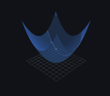
But our goal is to make the Error go down to zero! If increasing the weight makes the error go up, what should we do? We do the exact opposite of the slope. We need to subtract the slope from our current weight. This is called the Gradient Descent.
Gradient Descent looks like this:
The learning rate is there so that we don't take steps that are too big, to the point that we cross the entire valley.
In math, it looks like this:
Remember our chain rule equation we derived earlier:
Let's plug that slope into our Gradient Descent equation:
Look closely at what happens to the negative signs. You are subtracting a negative number. Those two minus signs cancel each other out and become a plus!
Also, remember that
So with some clean up, we get this:
Which, you may have noticed, is our weight update rule.
If the node is in the steep middle zone, the little slope ($S'$) is high, and the weight is allowed to update normally.
Enhancing Backpropagation
Vanilla gradient descent with a fixed learning rate is slow and gets trapped in shallow valleys of the error surface. Three classical refinements address this:
Momentum. A fraction of the previous weight update is added to the current one:
where
Adaptive Learning Rates (Delta-Bar-Delta). Rather than picking one
- If a weight's gradient direction is consistent across recent updates, increase its learning rate (we're confident, take bigger steps).
- If a weight's gradient keeps oscillating, decrease its learning rate (we're overshooting, slow down).
Modern variants of this idea (Adam, RMSProp) are still the default in deep learning today.
Quickprop. A second-order method that approximates the error surface near the current point as a parabola in each weight, then jumps directly to the parabola's minimum. When the assumption holds, Quickprop converges in dramatically fewer epochs than vanilla gradient descent.
6. Applications of Neural Networks
Neural networks excel in environments where data is noisy, relationships are non-linear, and traditional algorithmic logic fails.
General Functional Categories
- Clustering (Unsupervised): Exploring similarities between data patterns and grouping them. Use cases include data compression and data mining.
- Classification / Pattern Recognition: Assigning an input pattern (e.g., a handwritten symbol or an image) to one of many predefined classes.
- Function Approximation: Finding an estimate of an unknown mathematical function
subject to noise. This is heavily used in scientific and engineering disciplines. - Prediction / Dynamical Systems: Forecasting future values of time-sequenced data. Unlike standard function approximation, prediction incorporates the element of time, meaning the system state changes dynamically.
Specific Real-World Applications
- Medical Diagnosis:
- Input: Patient manifestations (symptoms, lab results, blood tests).
- Output: Predicted disease states (e.g., probability of prostate cancer or Hepatitis B).
- Advantage: Circumvents the need for explicit causal rules, which are often impossible to define in complex human biology.
- Process Control:
- Input: Environmental parameters and sensor readings.
- Output: Automated control parameters (e.g., adjusting valves, regulating temperature).
- Advantage: Learns ill-structured control functions that are too mathematically complex for standard PID controllers.
- Financial Forecasting:
- Input: Macroeconomic factors (CPI, interest rates) and historical stock quotes.
- Output: Forecasts of future stock prices or major indices (like the S&P 500).
- Consumer Credit Evaluation:
- Input: Personal financial metrics (income, debt-to-income ratio, payment history).
- Output: Risk assessment or credit rating scores.
7. Evaluation of Backpropagation Networks
While Multi-Layer Perceptrons trained with Backpropagation are exceptionally powerful, the architecture has both distinct advantages and inherent limitations.
Strengths
- Great Representation Power: The inclusion of non-linear hidden layers allows the network to approximate virtually any continuous function.
- Wide Practical Applicability: Easily adapted to classification, regression, and prediction tasks across countless domains.
- Easy to Implement: The calculus behind backpropagation is complex, but the algorithmic implementation is straightforward matrix multiplication.
- Good Generalization: When trained correctly (often utilizing cross-validation testing), ANNs can make highly accurate predictions on entirely unseen data.
Limitations and Problems
- Slow Convergence: Gradient descent can require tens of thousands of epochs (passes through the data) to reach an acceptable error rate.
- The "Black Box" Problem: It is nearly impossible to inspect the thousands of weights to understand why the network made a specific decision.
- Local Minima: Gradient descent only guarantees finding a local minimum error, not necessarily the global minimum.
- Representational Limits: Not absolutely every conceivable function can be learned easily within standard operational timeframes.
- Overfitting / Poor Generalization: If trained too long, the network may memorize the training data, leading to a situation where the training error is zero, but the network fails entirely on new data. Cross-validation is strictly required to prevent this.
- Lack of Quality Assessment: There is no mathematically well-founded way to assess the absolute quality of the learning aside from empirical testing on a hold-out set.
- Network Paralysis: If weights become too large, activation functions are driven into deep saturation regions. The derivatives become near zero, freezing the network.
- Trial-and-Error Architecture: Selecting the optimal learning rate, momentum, number of hidden layers, and nodes is still largely an empirical art rather than an exact science.
- Catastrophic Forgetting (Non-incremental Learning): Standard BP networks cannot easily learn "new" data on the fly. To incorporate new samples without forgetting old patterns, the network usually must be entirely retrained on the combined dataset.