What Even Is "Learning"?
Before we talk about machine learning, let's think about what learning means in general.
Herbert Simon, a Nobel Prize-winning scientist, once described learning as any process by which a system improves its performance from experience. That's a beautifully simple definition, and it applies just as well to computers as it does to humans.
When we talk about learning in the context of machines, the "tasks" we want them to improve at generally fall into two buckets:
- Classification — assigning things to categories (e.g., "Is this email spam or not?")
- Problem solving / Planning / Control — taking actions to achieve a goal (e.g., "How should a robot navigate a maze?")
Where Does Machine Learning Fit in the AI Landscape?
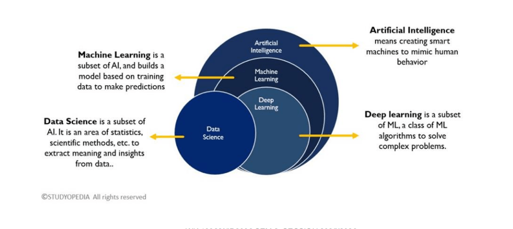
You've probably heard the terms AI, Machine Learning, Deep Learning, and Data Science thrown around interchangeably. They're related, but they're not the same thing.
Think of it as a set of nested circles:
- Artificial Intelligence (AI) is the broadest concept. It's about creating machines that can mimic intelligent human behaviour.
- Machine Learning (ML) is a subset of AI. Instead of being explicitly programmed with rules, ML systems learn patterns from data and use those patterns to make predictions or decisions.
- Deep Learning (DL) is a subset of ML that uses multi-layered neural networks to tackle complex problems like image recognition and natural language processing.
- Data Science overlaps with all of these. It's the broader discipline of extracting insights from data using statistics, scientific methods, and algorithms. The key takeaway: ML is about building models from training data to make predictions, rather than writing rules by hand.
The Main Flavours of Machine Learning
Machine learning approaches can be grouped into several categories based on how the system learns:
Supervised Learning — The model learns from labeled examples. You give it inputs paired with the correct outputs, and it learns the mapping between them. This includes regression (predicting a continuous value, like house prices) and classification (predicting a category, like spam vs. not spam).
Unsupervised Learning — The model receives data without labels and must find structure on its own. The most common task here is clustering — grouping similar data points together.
Reinforcement Learning — The model learns by interacting with an environment. It takes actions, receives rewards or penalties, and gradually figures out the best strategy. Think of it like training a dog with treats.
Self-Supervised Learning — A newer paradigm where the model generates its own labels from the data itself (for example, masking a word in a sentence and learning to predict it).
Real-World Applications
Classification Examples
Classification is everywhere in daily life:
- Medical diagnosis — Is this X-ray showing signs of pneumonia?
- Spam filtering — Should this email go to your inbox or junk folder?
- Fraud detection — Is this credit card transaction suspicious?
- Recommendation systems — Which movies, books, or songs might you enjoy?
- Speech and handwriting recognition — Converting spoken words or handwritten text into digital text.
Problem Solving / Planning / Control Examples
These are tasks where an agent takes actions in an environment to achieve a goal:
- Playing board games like chess or checkers
- Self-driving cars navigating roads
- Controlling robots or video game characters
- Flying drones or helicopters autonomously
Defining a Learning Task: T, P, E
One of the most useful frameworks for thinking about ML problems comes from Tom Mitchell's classic definition. Every learning task can be described by three components:
- T (Task) — What is the system trying to do?
- P (Performance) — How do we measure success?
- E (Experience) — What data does the system learn from? Here are a few examples to make this concrete:
| Task (T) | Performance (P) | Experience (E) |
|---|---|---|
| Playing checkers | % of games won | Self-play practice games |
| Recognizing handwritten words | % of words correctly classified | Database of labeled handwriting images |
| Driving on highways | Average distance before a human-judged error | Recorded images and steering commands from a human driver |
| Spam classification | % of emails correctly classified | Database of emails with human labels |
This framework is great for getting clarity before you start any ML project. Ask yourself: What's my T, P, and E?
Designing a Learning System
When you set out to build an ML system, there are four key design decisions:
- Choose the training experience — What kind of data will the system learn from? Is it direct (labeled input-output pairs) or indirect (like game outcomes where individual moves aren't labeled)?
- Choose the target function — What exactly should the system learn? For a checkers player, this might be an evaluation function that scores how favorable a board position is.
- Choose a representation — How will the target function be expressed? Options include lookup tables, linear functions, decision trees, neural networks, and many more.
- Choose a learning algorithm — How will the system search for the best function? This could be gradient descent, dynamic programming, evolutionary algorithms, etc.
A Concrete Example: Learning to Play Checkers
To tie everything together, let's walk through a classic example: Arthur Samuel's checkers-playing program from 1959, one of the earliest ML systems ever built.
The Target Function
We want to learn an evaluation function
if is a winning position if is a losing position if is a draw - Otherwise,
equals the value of the best reachable final state under optimal play
The problem? Computing this perfectly requires searching the entire game tree, which is astronomically large. So we need an approximation.
A Linear Approximation
We can represent the evaluation function as a weighted sum of board features:
Where:
= number of black pieces = number of red pieces = number of black kings = number of red kings = number of black pieces under threat = number of red pieces under threat
The weights (
Training with Indirect Experience
Since we're learning from self-play, we don't have direct labels for every board position. Instead, we use temporal difference learning: the estimated value of a board position is updated to be closer to the estimated value of the next board position in actual play. Over many games, accurate values from end-game positions gradually "back up" to earlier positions.
The LMS (Least Mean Squares) Algorithm
To adjust the weights, we use gradient descent. For each training example:
- Compute the error:
- Update each weight:
Here,
Deriving LMS
Let's take the guess from our AI, and call it
AI is just taking an approximation here, or just guessing random number, we can't really tell, so we can't rely on it entirely.
So, we define another variable,
And the raw mistake is just
Let's place
Now, we need a way to tell AI how bad it is doing overall. That's our cost function, let's call it
But this creates a problem: A huge positive error (guessing too low) and a huge negative error (guessing too high) will cancel each other out, making it look like the model is doing a great job when it isn't.
By squaring the error:
...we ensure that all errors are positive, and larger errors are heavily penalised.
When you use calculus to find the derivative (gradient) of that squared error equation to figure out how to adjust the weights, the 2 from the exponent drops down, cancels out the
Your mission is now to make J as close to zero as possible.
You might ask, why is
allowed here? As our aim is to minimise
(turning it to 0), although we are halving the hill's height and the gradient here, but it doesn't matter as long as we can get to the bottom of the hill. And we also utilise a learning rate later in the equation too, which can be anything the user wants to be. So this gets absorbed into the learning rate anyways.
To make J smaller, you have to tweak your weights (
You ask: "If I bump up a specific weight (
So, you take the derivative of your Cost function with respect to that specific weight:
Learn more about partial derivatives here.
Now we can use chain rule on our cost function.
Outside:
Inside: The guess
Multiply the outside and the inside together, and you get the gradient:
Which we can write simply as:
The gradient tells you the slope of the error. If the slope is positive, increasing the weight makes the error worse.
Since you want to minimize the error, you must do the exact opposite of what the gradient tells you. You subtract it! You also multiply it by a tiny learning rate (
Now, plug in the gradient you just found:
The two negatives cancel out into a positive, leaving you with:
How do we get
The LMS math works perfectly, but it relies entirely on having
There is no human sitting there labelling every single move with a perfect 1 to 100 score.
So, how does the AI generate its own
The AI doesn't know the exact value of a mid-game board, but the rules of Checkers provide an absolute, undeniable mathematical truth at the very end of the game. These are called Terminal States:
- Win = 100
- Loss = −100
- Draw = 0
The AI is not allowed to guess the score of a Terminal State. The game environment forces these numbers to be the absolute truth. Everything the AI learns is anchored to these final outcomes.
Temporal Difference (TD) Learning
Since the AI lacks a true
This is Temporal Difference learning. The AI essentially says: "I have better, more updated information after making a move than I did before making it. Therefore, my guess for the next state is a better target than my current guess."
How it works in practice:
- The Guess: At Step 4, the AI evaluates the board and guesses a score of 90.
- The Move: The AI makes a move and immediately wins the game (Step 5).
- The Correction: The environment declares Step 5 is a Terminal State worth 100.
- The Update: The AI looks back at Step 4. It realizes its guess of 90 was wrong, because Step 4 directly led to a 100. It sets
for Step 4 to 100, and the LMS algorithm kicks in to adjust the weights up. - The Win (Pushing Up): Let's say the AI evaluates the state at 90. It wins, so the target is 100.
- Error=+10
- Adjustment=0.1⋅10=+1
- New Value = 91 (It steps towards 100, but doesn't jump all the way there).
- The Loss (Dialling Back): The next game, it reaches that same state, confidently guesses 91, but falls into a trap and loses. The target is now −100.
- Error=−100−91=−191
- Adjustment=0.1⋅(−191)=−19.1
- New Value = 71.9 (It takes a massive hit and dials way back).
Over thousands of games, the absolute certainty of the end-game (100 or -100) slowly ripples backward through the moves. Step 4 learns from the Win, then Step 3 learns from Step 4, and so on. Eventually, the evaluation function perfectly maps out the true probability of winning from any starting board state.
The intuition is simple:
- If the prediction is correct → no change
- If the prediction is too high → decrease weights proportionally
- If the prediction is too low → increase weights proportionally
Under reasonable conditions, LMS is guaranteed to converge to the weights that minimise the Mean Squared Error (MSE):
Understanding the formula
This formula is really just an ultimate scoreboard for AI.
Mean:
Squared:
Error:
It adds up all the errors, and find the average error rate so that you can compare it between models.
Training Data: Where Does It Come From?
The source and nature of training data matters a lot. A few scenarios:
- Random examples provided by the environment (most common in practice)
- Teacher-selected examples chosen to be maximally informative (like "near-miss" examples)
- Active learning where the model queries an oracle / human for labels on examples it's unsure about
- Self-directed experimentation where the learner designs its own experiments
A key assumption in most ML is that training and test data are independently and identically distributed (IID) — drawn from the same underlying distribution. When this assumption breaks down, you need techniques like transfer learning (different distributions) or collective classification (non-independent examples).
What is IID? (Independently and Identically Distributed)
IID is a mathematical assumption that ML models make about the world. It assumes your training data and your real-world test data are perfectly consistent. Let's split it into its two halves:
1. "Independently"
This means that one piece of data has absolutely no connection to the next piece of data. Drawing one doesn't change the probability of the next.
- IID (Independent): Rolling a die. Rolling a 6 doesn't change the odds of rolling a 6 on the next turn. Diagnosing patients in a clinic; Patient A having a cold doesn't magically make Patient B have a broken leg.
- NOT Independent: Predicting the weather. If it is raining on Tuesday, it is highly likely to be raining on Wednesday. The data points are linked in time.
2. "Identically Distributed"
This means all your data is pulled from the exact same "world," under the exact same rules, conditions, and demographics.
- IID (Identical): Training an AI to grade math tests from a specific school, and testing it on different math tests from that same school.
- NOT Identical: Training a self-driving car entirely on the sunny, wide streets of Phoenix, Arizona (Training Data), and then dropping it into a blizzard in the narrow streets of Boston (Test Data). The "distribution" of the data—the weather, the roads, the driver behavior—has completely changed.
When an AI model is trained, it only learns the exact rules of its training data. If the real world is not IID to the training data, the AI will confidently make terrible predictions.
What is Transfer Learning?
(The fix for when data is NOT Identically Distributed)
Let's say the "Identically Distributed" assumption breaks. You want to build a medical AI to detect a very rare disease in X-rays. Because the disease is rare, you only have 100 training images. That isn't enough to train a neural network from scratch.
Transfer Learning is the process of taking a model trained on a massive, different dataset, and "transferring" its foundational knowledge to your new problem.
- You take a model that Google already trained on 10 million random internet images (cats, dogs, cars, trees). This model already knows how to detect edges, shapes, textures, and shadows.
- You take that pre-trained model and do a little bit of extra training using your 100 rare X-rays.
- The model transfers its general knowledge of shapes and textures to the specific task of reading X-rays.
It saves massive amounts of time and data when your target environment doesn't match a massive, easily available training environment.
What is Collective Classification?
(The fix for when data is NOT Independent)
Let's say the "Independent" assumption breaks. Your data points are heavily connected to one another, usually in a network or a graph.
Imagine you are trying to catch bot accounts on a social media platform. If you look at an account strictly in isolation (its bio, its profile picture, its post frequency), you might not be able to tell if it's a bot.
However, in a social network, users aren't independent. Collective Classification is a technique that looks at the relationships between data points.
- If Account A follows 500 known bots.
- If Account A is followed by 500 known bots.
- Collective Classification uses the known labels of the neighbors to classify the target. It concludes Account A is almost certainly a bot, too!
To sum up your notes: IID is the "perfect laboratory condition" for an AI. Transfer Learning and Collective Classification are the rescue tools you use when those perfect conditions shatter in the real world.
How We Represent Target Functions
Different representations offer different trade-offs between expressiveness and learnability:
Numerical functions — linear regression, neural networks, support vector machines. These are great at capturing smooth, continuous patterns.
Symbolic functions — decision trees, logical rules. These produce human-interpretable models.
Instance-based functions — nearest-neighbor, case-based reasoning. These make predictions by comparing new examples to stored training examples.
Probabilistic graphical models — Naïve Bayes, Bayesian networks, Hidden Markov Models. These explicitly model uncertainty and dependencies between variables.
The more expressive a representation, the more complex functions it can capture — but it also needs more data to learn accurately. This is a fundamental trade-off in ML.
Evaluating Learning Systems
How do we know if a learning system is actually good? There are two main approaches:
Experimental evaluation — Run controlled experiments using cross-validation on benchmark datasets. Measure things like test accuracy, training time, and testing time. Use statistical tests to determine whether differences between methods are meaningful.
Theoretical analysis — Prove mathematical guarantees about algorithms, such as computational complexity, the ability to fit data, and sample complexity (how many examples are needed to learn well).
In practice, most ML work uses a combination of both.
A Brief History of Machine Learning
ML has a rich history spanning several decades:
- 1950s — Samuel's checkers player at IBM, one of the first programs to learn from experience
- 1960s — The Perceptron (an early neural network), and Minsky & Papert's proof of its limitations
- 1970s — Symbolic approaches take center stage: decision trees (ID3), expert systems, and scientific discovery programs
- 1980s — Neural networks make a comeback with backpropagation; PAC learning theory provides mathematical foundations
- 1990s — Data mining, reinforcement learning, ensemble methods (bagging, boosting), and Bayesian approaches
- 2000s — Support vector machines, kernel methods, transfer learning, and ML applications in security, robotics, and personalization And of course, from the 2010s onward, deep learning has transformed the field — but that's a story for later weeks!
Key Takeaways
- Machine learning is about learning from experience — using data to approximate functions, rather than coding rules by hand.
- Every ML problem can be framed as T, P, E — the task, the performance metric, and the experience.
- Designing an ML system involves four choices: training experience, target function, representation, and learning algorithm.
- There's always a trade-off between model expressiveness and the amount of data needed.
- Evaluation matters — a model is only as good as its performance on unseen data.