What Is a Decision Tree?
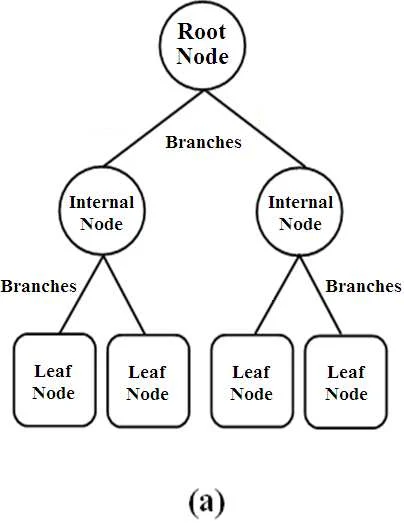
A decision tree is exactly what it sounds like — a tree-shaped model that makes decisions. Each internal node asks a question about a feature, each branch represents a possible answer, and each leaf gives you a final classification.
Here's a classic example: should you play tennis today?
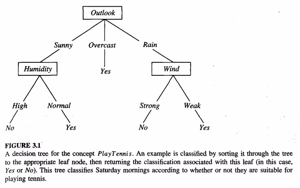
The tree checks the weather outlook first. If it's overcast, just go play — always yes. If it's sunny, check the humidity. If it's rainy, check the wind. Simple and readable.
We can also express this tree as a set of logical rules (called disjunctive normal form):
Yes Yes Yes
This is one of the best things about decision trees, you can always convert them into human-readable if-then rules.
Why Decision Trees?
Decision trees have several properties that make them a solid starting point for classification problems:
- They handle both discrete and continuous features. Discrete features like color (red, blue, green) work naturally. For continuous features like temperature, the tree can split on a threshold (e.g., temperature < 30°C vs. ≥ 30°C).
- They naturally represent disjunctive (OR) concepts. Some classification boundaries are complex unions of conditions, but decision trees handle this natively.
- They're robust to noise. Both mislabeled examples and noisy feature values can be tolerated.
- They handle missing values. If a data point doesn't have a value for some feature, the algorithm can still work with it.
- Classification trees produce discrete class labels at the leaves, while regression trees output continuous real-valued predictions.
How Do We Build a Decision Tree?
The core algorithm is a top-down, recursive, divide-and-conquer approach. Here's the pseudocode:
DTree(examples, features):
    If all examples belong to one class:
        return a leaf with that class label

    If no features are left:
        return a leaf with the majority class

    Pick the "best" feature F
    Create a node for F
    For each value v of F:
        Let examples_v = subset of examples where F = v
        If examples_v is empty:
            attach a leaf with the majority class of examples
        Else:
            attach DTree(examples_v, features - {F})

    Return the tree rooted at this node
The key question is: how do we pick the "best" feature?
Pseudocode Explaination
1. Check the Stopping Rules (Base Cases)
Before trying to split the data, the algorithm checks if it should stop growing the tree:
- Pure Data:
If all examples belong to one class:If every item in the current dataset belongs to the exact same category (e.g., they are all "Spam"), it stops and creates a leaf node predicting that exact category.- > Are all the fruits in the basket apples? No, it’s a mix.
- Out of Features:
If no features are left:If the algorithm has used up all the available features to split on, but there are still mixed classes in the dataset, it stops. It creates a leaf node predicting the majority class (whichever category is most common in that remaining subset).- Have we run out of questions to ask? No, we still have Size and Color.
2. Choose the Split (The Divide Step)
If the algorithm hasn't stopped, it needs to figure out how to divide the data:
Pick the "best" feature F:It evaluates all available features and chooses the one that best separates the classes.- The algorithm evaluates Size and Color to see which question separates the fruits best. Let's say it determines that asking about Size is the best first move, because it easily separates the grapes from the larger fruits.
Create a node for F:It makes this chosen feature a decision point (a node) in the tree.- It creates the very first decision point (the root node) in our tree: "What is the Size?"
3. Split the Data and Repeat (The Conquer Step)
Once the best feature is chosen, the algorithm branches out:
For each value v of F:It creates a branch for every possible answer to the feature's question (e.g., if the feature is "Weather", the branches might be "Sunny", "Rainy", and "Cloudy").Let examples_v = subset...:It divides the current dataset, sending the relevant examples down their respective branches.- It gathers all the "Small" fruits into a new subset.
- Handle Empty Branches:
If examples_v is empty:If a branch ends up with absolutely no data, the algorithm doesn't crash; it simply caps that branch with a leaf node predicting the majority class of the parent data. - Recursion:
Else: attach DTree(...)If the branch does have data, the algorithm calls itself to repeat the exact same process on this new, smaller subset of data, using only the features that haven't been used yet (features - {F}).- It runs the algorithm again on just the small fruits.
- Recursion kicks in: When looking at this "Small" subset, it realizes every single fruit here is a Grape! It hits the first stopping rule (If all examples belong to one class) and instantly creates a Leaf: Grape.
4. Return the Result
Return the tree rooted at this node:Finally, it passes the fully assembled sub-tree back up the chain until the entire decision tree is built.- The algorithm stitches all these sub-trees and leaves together. It passes the finished flowchart back to you:
- First, check Size.
- If Small ➔ It's a Grape.
- If Big ➔ Check Color.
- If Red/Green ➔ It's an Apple. If Yellow ➔ It's a Lemon.
- The algorithm stitches all these sub-trees and leaves together. It passes the finished flowchart back to you:
Entropy and Information Gain
This is where information theory comes in. We want to choose the feature that best separates the data — the one that brings us closest to pure (single-class) subsets.
Entropy
Entropy measures the impurity or disorder of a set. For a binary classification:
where
Some intuition:
- If all examples are the same class → entropy = 0 (perfectly pure, no uncertainty)
- If examples are evenly split (50/50) → entropy = 1 (maximum uncertainty)
Let's break down this equation piece by piece.
1. The Fractions (
is the fraction of the basket that is Apples. If you have 10 fruits and 7 are Apples, . is the fraction that is Lemons. In that same basket, 3 are Lemons, so . (Note: and must always add up to 1, representing 100% of the basket).
2. The Logarithm (
Why use a base-2 logarithm? It measures "bits" of information. Think of it as asking: "How many yes/no questions (bits) would I need to ask to figure out the identity of a randomly picked fruit?"
The log of a fraction (any number between 0 and 1) is always a negative number.
3. The Negative Sign (
Because the logarithm of a fraction gives us a negative number, calculating
Why is this useful for Decision Trees?
When the algorithm is picking the "best" feature to split the data (from step 2 of our pseudocode), it calculates the entropy before the split, and compares it to the entropy after the split.
If asking "Is the fruit Big?" drops the entropy from 1.0 (a total mess) down to 0.2 (mostly organized), that means it's a fantastic question to ask! This drop in entropy is exactly what we call Information Gain.
For multi-class problems with
You can think of entropy as the average number of bits needed to encode the class label of a randomly chosen example — more uncertainty means more bits.
Information Gain
Information gain measures how much entropy decreases after we split on a particular feature:
where
In plain language: information gain = entropy before the split − weighted average entropy after the split. The feature with the highest information gain wins.
1. Multi-Class Entropy
The Equation:
The Explanation: This is the exact same equation as the binary one you saw earlier, just generalized so it works for any number of categories, not just two.
: This just means "add everything together." : The total number of classes. In our previous example (Apples, Lemons, Grapes), . : The fraction of the dataset that belongs to class .
So, instead of just calculating
2. Information Gain
The Equation:
The Explanation:
This equation is the brain of the decision tree. It calculates exactly how good a specific feature (
: This is the messiness of your data before you split it. ( stands for the original Set of data). - The Subtraction (
): We are taking the messiness before the split, and subtracting the messiness after the split. If the number goes down a lot, our "Gain" is high. : This just means "for every branch we create." If the feature is "Color", then represents "Red", "Green", and "Yellow". : This is the messiness of the data inside one specific branch (e.g., how messy is the "Red" pile?). (The Weight): The straight bars mean "count". is the number of items in this specific branch, and is the total number of items overall. This creates a fraction (e.g., 4 items out of 10 = ).
Why do we need the weight?: Imagine you have 100 fruits. You ask a terrible question: "Does the fruit have exactly 341 tiny dimples on its skin?"
- Branch 1 (Yes): Only 1 fruit goes here. It happens to be an Apple. The entropy of this branch is 0 (perfectly pure!).
- Branch 2 (No): 99 fruits go here. It's a complete, jumbled mess of Apples, Lemons, and Grapes. The entropy is very high.
If we just averaged the two entropies together, the 1-fruit branch would artificially make the split look really good. By multiplying by
- Branch 1 gets a weight of
(barely counts). - Branch 2 gets a weight of
(counts heavily).
Bringing it all together:(Messiness of Parent) MINUS (Weighted Average Messiness of the Children).
When the decision tree is sitting at Step 2 of the pseudocode ("Pick the best feature"), it calculates this exact Information Gain equation for Size, and then for Color. Whichever feature gives the highest number (meaning it removed the most messiness) is the winner, and becomes the next node in the tree!
A Worked Example
Consider four examples with features (size, color, shape) and a binary class (+/−):
| Example | Size | Color | Shape | Class |
|---|---|---|---|---|
| 1 | big | red | circle | + |
| 2 | small | red | circle | + |
| 3 | small | red | square | − |
| 4 | big | blue | circle | − |
The overall dataset has 2 positives and 2 negatives, so
Splitting on Size:
- big → 1+, 1− →
- small → 1+, 1− →
— useless!
Splitting on Color:
- red → 2+, 1− →
- blue → 0+, 1− →
— much better.
Splitting on Shape:
- circle → 2+, 1− →
- square → 0+, 1− →
— tied with color.
So we'd pick either color or shape first (both have gain = 0.311), and definitely not size (gain = 0).
The ID3 Algorithm
The algorithm we've been describing is called ID3, invented by J. Ross Quinlan in 1979. It uses Shannon's information theory (1948) to select features via information gain. Key characteristics:
- Builds the tree top-down with no backtracking (the algorithm is stubbornly committed to its choices, greedy algorithm)
- Selects the feature with the highest information gain at each step
- Runs recursively on non-leaf branches until all data is classified
- Searches the entire dataset to construct the tree Later improvements led to C4.5 (Quinlan, 1993), which handles continuous attributes, missing values, and pruning. Another parallel development was CART (Classification and Regression Trees) by Breiman and Friedman.
A Fun Example: Classifying Simpsons Characters
Let's say we want to classify Simpsons characters as Male or Female using three features: hair length, weight, and age.
| Person | Hair Length | Weight | Age | Class |
|---|---|---|---|---|
| Homer | 0" | 250 | 36 | M |
| Marge | 10" | 150 | 34 | F |
| Bart | 2" | 90 | 10 | M |
| Lisa | 6" | 78 | 8 | F |
| Maggie | 4" | 20 | 1 | F |
| Abe | 1" | 170 | 70 | M |
| Selma | 8" | 160 | 41 | F |
| Otto | 10" | 180 | 38 | M |
| Krusty | 6" | 200 | 45 | M |
The dataset has 4 females and 5 males, with
We compute the information gain for splitting on each feature:
- Hair Length ≤ 5? → Gain = 0.0911
- Weight ≤ 160? → Gain = 0.5900 ← Winner!
- Age ≤ 40? → Gain = 0.0183 Weight gives us the best split. Everyone over 160 lbs turns out to be male (entropy = 0 on that branch — done!). But the ≤160 group still has a mix (4F, 1M), so we recurse.
On the second split, we find that Hair Length ≤ 2 perfectly separates the remaining group: Bart (short hair, male) vs. the females (longer hair).
The final tree:
            Weight ≤ 160?
            /           \
          yes            no
          /               \
   Hair Length ≤ 2?      Male
      /        \
    yes         no
    /             \
  Male          Female
And as rules:
- If Weight > 160 → Male
- Else if Hair Length ≤ 2 → Male
- Else → Female Now if Comic Book Guy shows up (Hair: 8", Weight: 290, Age: 38), the tree says: Weight 290 > 160 → Male. Correct!
The Overfitting Problem
Here's the catch: a tree that perfectly classifies every training example isn't necessarily a good tree.
Overfitting happens when a model fits the training data too well — including its noise and quirks — and performs poorly on new, unseen data. Formally, hypothesis
Think of it this way: if you measure 10 data points for Ohm's Law (
The same thing happens with decision trees — noise in the data can cause the algorithm to create extra branches that capture randomness rather than real patterns.
How Noise Causes Overfitting
Imagine our color/shape example, and one training instance gets mislabeled. The tree might need to add extra splits on irrelevant features (like size) just to account for that one noisy data point. The result is a bigger, more complex tree that generalizes poorly.
Pruning: The Cure for Overfitting
There are two main strategies:
Prepruning — Stop growing the tree early, before it perfectly fits the training data. For example, stop when a node has too few examples to split reliably.
Postpruning — Grow the full tree first, then cut back branches that don't help generalization. This is generally more effective since it's hard to know when to stop growing.
Reduced Error Pruning
A common postpruning method:
- Split your data into a "grow" set and a "validation" set
- Build a complete tree from the grow set
- For each internal node, try replacing its subtree with a leaf (majority class)
- If the replacement improves accuracy on the validation set, make it permanent
- Repeat until no more pruning helps The downside is that you "waste" some training data on validation. An alternative is to run multiple trials with different random splits, average the resulting tree complexity, then grow a final tree from all the data up to that average complexity.
Other Pruning Approaches
- Statistical tests — Check whether the pattern at a node is statistically significant or just random chance
- Minimum Description Length (MDL) — Ask whether the extra tree complexity is worth it compared to just memorizing the exceptions
Computational Complexity
In the worst case (a complete tree testing every feature on every path), building a decision tree takes
In practice, the tree is rarely complete, and the complexity is roughly linear in both
Strengths and Limitations
Strengths
- Produces interpretable, human-readable rules
- Fast to build and fast to classify new instances
- Handles both categorical and numerical features
- Robust to noise and missing data
- No need for feature scaling or normalization
Limitations
- Prone to overfitting, especially with small datasets
- Tests only one feature at a time (axis-aligned splits) — can't easily capture diagonal decision boundaries
- Information gain has a bias toward features with many values
- Greedy construction doesn't guarantee the globally optimal tree (finding the smallest consistent tree is NP-hard)
- Produces a single deterministic hypothesis with no confidence estimates
What Comes Next?
Decision trees are a foundation for more powerful methods:
- Random Forests — build many decision trees on random subsets of features and data, then vote
- Gradient Boosted Trees (XGBoost, LightGBM) — build trees sequentially, each one correcting the errors of the previous
- C4.5 / C5.0 — Quinlan's improvements to ID3 with better handling of continuous features, missing values, and pruning These ensemble methods are among the most successful algorithms in practice, especially for structured/tabular data — and they all build on the decision tree concepts we've covered here.
These notes are based on Week 4 of WIA1006/WID3006 Machine Learning at Universiti Malaya (Semester 2, 2025/2026). If you found this helpful, stay tuned for more ML concepts explained from scratch!